Advanced Genetic Algorithms

The program AGA may be used to solve the great majority of the one-criterion optimisation problems. Short description of this program is presented below on the basis of two variables function optimisation.

(1)

given by

(2)

The smallest values

The easiest way to find that minimum is to write a script file in the following format

[VARIABLES]

x = real [0; 3.1415]

y = real [0; 3.1415]

[FUNCTION]

analytical = 1

[EQUATIONS]

f = -5.*sin(x)*sin(y) - sin(5*x)*sin(5*y)

[SHOW]

arrange = 1

[OPTIONS]

maximisation = 0

loop_counter = 100

max_iteration = 100

[SELECTION]

tournament = 1

tournament_size = 3

[CROSSOVER]

probability = 0.7

arithmetical = 1

[MUTATION]

probability = 0.15

nonuniform = 1

[POPULATION]

size = 30

constatnt = 1

[PLOTS]

Convergence = Average;CurrentMin

D = Discrepancy

Different_vs_2^Entropy = Different;2^Entropy

Save it as ‘test.txt’ and you can run it writing in your command line ‘aga test.txt’. Then you shall see something like this

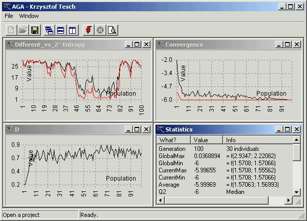
AGA found the infimum called ‘GlobalMin’ (see window named ‘Statistics’) . It is very close to the exact value. If you do not want to use the command line then fire up AGA and you see window

Choose option ‘Open’ from menu ‘File’ and then find your file ‘test.txt’ and choose ‘Open’.

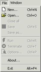
Instead of writing script file you can define your optimisation problem manually. To do this choose menu ‘File’

- ‘New...’ – click here if you want to define your problem

- ‘Open...’ – open your problem definition from file. There are two types of file

- *.txt – script files (text)

- *.aga - AGA internal files (binary)

- ‘Close all’ – closes all the windows and finish your optimisation

- ‘Save’ – save current problem

- ‘Save as…’ – save current problem with a different name

- ‘Run’ – run your optimisation process

- ‘Terminate…’ – terminate your running process

- ‘About…’ – short note about the author

- ‘Exit’ – exit application

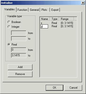
when you choose option ‘New’ from menu ‘File’ you will se dialog box called ‘Initialise’. Dialog box ‘Initialise’ is composed of five pages. First page ‘Variables’ is used to declare optimisation variables (in the case of function optimisation – independent variables).

There are three types of variables:

- ‘Boolean’ – logical variable. Two values are possible: 0 (false) and 1 (true).

- ‘Integer’ – integer variable. Values from the subset of integer numbers are possible. If an integer variable has been chosen it is necessary to specify the range of the desired subset. There are two edit windows: ‘from’ and ‘to’.

- ‘Real’ – floating point variable. Values from the subset of floating point numbers are possible. In this case also it is necessary to specify the range of the desired subset. There are two edit windows: ‘from’ and ‘to’. After filling them the range of the subset is given by .

When the edit windows ‘from’ and ‘to’ are filled, the next step is to add variables to the list. To do this: use a button ‘Add’. If you want to remove a variable from the list then highlight it and push ‘Remove’ button. If you want to name your variable just click on the empty place in the column ‘Name’. If the name is not specified the program will assume default name (x1, x2, …). In our case we can name our variables: x and y.

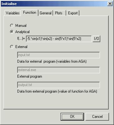
Second page control ‘Function’ of the dialog box ‘Initialise’ determines the entry method for the value fitness function. There are three possibilities:

- ‘Manual’ – enter individual values by hand

- ‘Analytical’ – you can specify analytical equation

- ‘External’ – automatically by external program (*.exe or *.bat file).

Manual entry of the value fitness function is required for all the values that are not calculated yet during the optimisation process step.

We decided to deliver value fitness function by analytical equation. To do this input in edit box ‘f(…)=’:

-5.*sin(x)*sin(y) - sin(5*x)*sin(5*y)

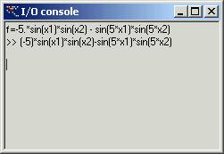
If description of the function is more complicated the you have to push button ‘I/O’ – that will open I/O console. For more precision description see ‘I/O Console’ paragraph. The function must be called ‘f’.

If you decide to deliver value fitness function from an external program, you must specify the name of the text file into which AGA will send independent variables that are generated by GA. The external program must calculate value of the function for these variables (‘Data for external program (variables from AGA)’). Default name of this file is ‘input.txt’. The name of executable (*.exe) program or *.bat file which is going to calculate these values must also be specified (‘External program’). The external program has to save the calculated value to another text file. That text file will be received by AGA to continue optimisation process (‘Data from external program (function value for AGA)’). Default name of this file is ‘output.txt’. This makes it possible to create a fully automated optimisation process. In our case example, the source code looks:

#include <fstream.h>

#include <math.h>

int main(int /*argc*/, char *argv[]) {

ifstream in(argv[1]);

ofstream out(argv[2]);

double x1, x2, f;

in >> x1 >> x2;

f = -5.*sin(x1)*sin(x2) - sin(5*x1)*sin(5*x2);

out << f << endl;

return 0;

}

It calculates the value of function given by equation (2). Source code listed above should be compiled and the executable version should be placed into the folder together with AGA.

Input data are received from the file specified as a first argument (argv[1]) and result saved into file specified as a second argument (argv[2]). The AGA program will call the external program with command-line arguments, using the syntax:

External.exe input.txt output.txt

Third page control ‘General’ allows you to choose population size and windows you want to see during optimisation process

- ‘Statistics history’ – you will see statistics for every iteration or for the last one (current) if it is unchecked

- ‘Buffer individuals’ – to save computation time you can buffer already calculated fitness function values. It works very well for integer and boolean variables.

- ‘Show buffered’ – shows buffered individuals with calculated fitness function values (if ‘Buffer individuals’ has been chosen)

- ‘Show population’ – shows individuals of last generation. It is important for manual delivering of fitness function. Then you have to input those values.

- ‘Population history’ – as above (if ‘Show population’ has been chosen) but it shows all the generations.

- ‘Show variables’ – displays basic information about optimisation variables

- ‘(Initial) population size’ – here you can specify the size of the population. For variable population size method it is initial population size only (first step).

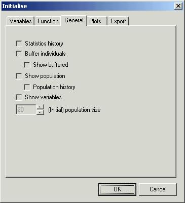
In our case set ‘(Initial) population size’ to 30.

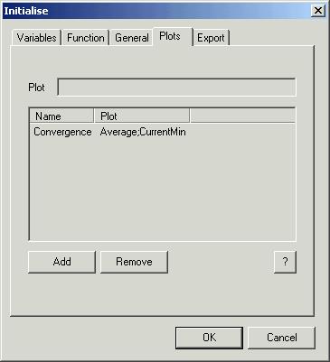
Fourth page control ‘Plots’ makes possible to specify the plots you want to see during optimisation process. One plot is predefined (for minimisation). It is plot called ‘Convergence’. The name you choose is inconsequential. If you do not name your plot then AGA will do it for you. To plot something you must input this in the window ‘Plot’ and push button ‘Add’. If you change your mind then remove it using button ‘Remove’.

You can plot variables or even equations. To remind yourself of the standard variable names push button ‘?’ and you will see the following window:

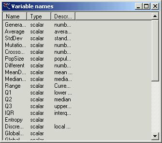
To input your equation use variable names specified in the first column of this window. If you want to see more than one plot in the same window the separate your equations using ‘;’. In our case you can add two additional plots. To do it input

Discrepancy

in the edit window ‘Plot’, push button ‘Add’ and then change the plot’s name to

The second plot is composed of two graphs that show the number of different individuals and the function . To do it input

Different;2^Entropy

and optionally change the name to

Different_vs_2^Entropy

Fifth page control ‘Export’ allows you to export variables or equations to file. The rules of exporting are the same as in page control ‘Plots’. There are two differences: you have to specify a single equation (do not use ‘;’ to separate) and you can export vector variables (instead of scalar for plotting).

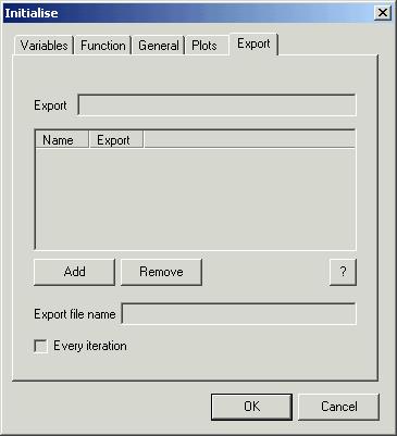
To choose the name of export file name input it to ‘Export file name’. Check box ‘Every iteration’ allows you to export results from each iteration, or from the last only if it is left unchecked.

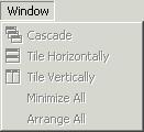
Menu ‘Window’ is composed of at least five options for windows manipulation

- ‘Cascade’

- ‘Tile Horizontally’

- ‘Tile Vertically’

- ‘Minimize All’

- ‘Arrange All’

The speed toolbar is composed of six buttons. They are:

- ‘New’ – same as option ‘New’ form menu ‘File’

- ‘Open’ – same as option ‘Open’ from menu ‘File’

- ‘Save’ – same as option ‘Save’ from menu ‘File’

- ‘Cascade’ – same as option ‘Cascade’ from menu ‘Window’

- ‘Tile Horizontally’ – same as option ‘Tile Horizontally’ from menu ‘Window’

- ‘Tile Vertically’ – same as option ‘Tile Vertically’ from menu ‘Window’

- ‘Run’ – same as option ‘Run’ from menu ‘File’

- ‘Terminate’ – same as option ‘Terminate’ from menu ‘File’

- ‘Options’ – same as options ‘Options’ from menu ‘File’

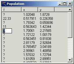
If you have decided to input function value manually then you have to supply these values in the window ‘Population’ for each set of independent variables listed out by the program. First click on the desired line and then click again on the ‘?’. Finally you can input a value.

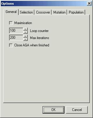
It is also possible to modify the optimisation process options. To do this choose either option ‘Options’ from menu ‘File’ or the relevant speed button. Dialog box ‘Options’ is composed of five pages. The first of them, labelled ‘General’ allows you to choose maximal number of iterations ‘Max iteration’ and change the number of generations ‘Loop counter’. The number of generations is important only for external and analytical method of supplying the function value. You can decide here whether you maximise or minimise your problem - ‘Maximisation’. AGA may optionally be closed when the optimisation is finished. To do this choose ‘Close AGA when finished’. It is useful when you call AGA from other program or want to fully automate your computation.

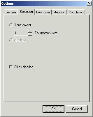
Second page ‘Options’ allows you to choose selection method. There are two methods so far:

- ‘Tournament’ – random tournament selection (default). You can specify the size of tournaments ‘Tournament size’. Default tournament size equals 3. Due to its virtues this method is recommended.

- ‘Roulette’ – roulette wheel selection. Roulette wheel method is a classical method of individual selection. It possesses more defects than virtues.

Both methods fits either maximisation or minimisation problems. It means that roulette method is modified version of classical roulette.

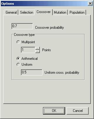
Third page ‘Crossover’ contains options that are necessary to change crossover method. One can also change ‘Crossover probability’. There are three crossover methods

- ‘Multipoint’ – multipoint method. ‘Points’ indicates the number of crossover points. Default number is 1.

- ‘Arithmetical’ – arithmetical crossover method. This method is suitable for numerical optimisation.

- ‘Uniform’ – exchanges all the genes with ‘Uniform cross probability’

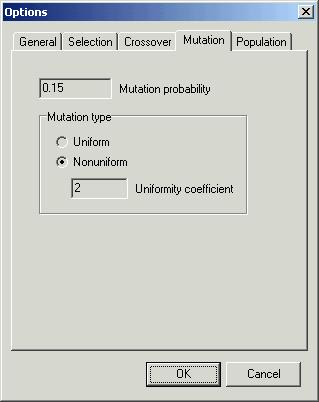
Fourth page ‘Mutation’ allows you to specify ‘Mutation probability’ and to choose among mutation methods

- ‘Uniform’ – this method does not depend on current generation number (stage of optimisation)

- ‘Nonuniform’ – this method depends on current generation number. The later the generation the smaller the influence of mutation. You can also change the ‘Uniformity coefficient’.

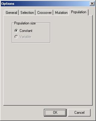
Fifth page ‘Population’ lets you to choose population size. There are two possibilities

- ‘Constant’ – population size does not depend on generation number – is constant during optimisation process

- ‘Variable’ – population size varies during optimisation process.

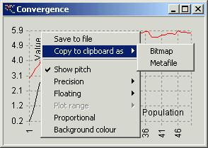
Right mouse button clicked on chart window displays popup menu. This menu allows you to modify your chart.

- ‘Save to file’ – save the chart as bitmap to file

- ‘Copy to clipboard as’ – copies the chart to clipboard as

- ‘Bitmap’

- ‘Metafile’ – enhanced metafile (‘emf’ format)

- ‘Show pitch’ – shows or hides chart pitch

- ‘Precision’ – sets number of decimal digits along specified axis

- ‘x’

- ‘y’

- ‘Floating’ – allows you to change floating number to integer on specified axis

- ‘x’

- ‘y’

- ‘Plot range’

- ‘Proportional’ – makes the chart proportional. It is useful when x-axis and y-axis are similar or the same

- ‘Background colour’ – changes the background colour of your chart

I/O Console

There is a difference between capital and small letters! When a function does not give unique value then the main value is returned. You operate on tensors in general. Scalars are zero valence tensors. Complex numbers are represented in the form of

a + b*I

where ‘a’ is real part and ‘b’ imaginary part. Real parts are represented as double precision 64 bits number. Space characters are ignored.

If input value can be transformed into numerical value then AGA returns numerical value. For instance

2 + pi / e

gives

3.15573

if input value cannot be transformed to numerical value then AGA will try to simplify its part and will treat it as symbolic value. For instance

2 * pi / x

gives

6.28319/x

under condition that you have not defined x yet.

Commands are characterised by square brackets [] and cannot be nested.

Command list:

- ‘List[]’ – lists all declared and predefined variables. Predefined variables are

- pi =

- deg =

- Generation – generation number

- Average – average fitness function

- StdDev – standard deviation

- Mutations – mutations number

- Crossovers – crossovers number

- PopSize – population size

- Different – number of different fitness function values

- MeanDev – mean deviation

- MedianDev – median deviation

- Range = CurrentMax – CurrentMin

- Q1 – lower quartile

- Q2 – median

- Q3 – upper quartile

- IQR = Q3-Q2 – interquartile range

- Entropy

- Discrepancy

- GlobalMax – maximal fitness function value from all generations

- GlobalMin – minimal fitness function value from all generations

- CurrentMax – maximal fitness function value from current generation

- CurrentMin – minimal fitness function value from current generation

- CrossPoints – number of crossover points

- TourSize – tournament size

- Buffered – number of buffered individuals

- CrossUnifProb – uniform crossover probability

- CrossProb – crossover probability

- MutProb – mutation probability

- GlobalMinIndiv – individual with minimal fitness function value from all generations

- GlobalMaxIndiv – individual with maximal fitness function value from all generations

- CurrentMinIndiv – individual with minimal fitness function value from current generation

- CurrentMaxIndiv – individual with maximal fitness function value from current generation

- ‘Clear[]’ – clears all declared variables

- ‘Clear[x]’ – clears x variable

Functions are characterised by round brackets (). Three dots in (...) mean that it is a function with variable number of arguments. All the functions can be nested as many times as you want.

Function list:

vect(...) vect function lets you input tensor of valence described by square number. For instance: first valence tensor is just a vector. To obtain vector composed of three coordinates a, b, c you must write

vect(a, b, c)

There is a shorter and more comfortable way of inputting tensors by means of curly brackets. Previous example now looks like this

{a, b, c}

Second valence tensor - matrix looks like this

{{A, B, C}, {D, E, F}}

in traditional notation

matrix

{{A, B}, {C, D}, {E, F}}

in tradition notation

sin() calculates sine function. Arguments ought to be given in radians. To convert degrees to radians multiply them by deg. For example

sin(45 * deg)

gives or numerically

0.707107

It is possible to calculate sine of complex arguments or of objects different than scalars. For instance sine of a vector

sin({I, pi, a})

gives the vector

{1.1752*I,1.22515e-16,sin(a)}

that is sine of all components. If argument is symbolic then results are symbolic as well.

cos()

tg()

ctg()

sinh()

cosh()

tgh()

ctgh()

arcsin() calculates arcus sine of complex argument. Result is given in radians. To convert to degrees divide it by deg. For instance for the angle equals

arcsin(sqrt(2) / 2) / deg

gives

arccos()

arctg()

arcctg()

arsinh()

arcosh()

artgh()

arctgh()

log(,) log(a, b) calculates logarithm of b to base a. If results of this operation is c then a^c == b. For instance

log(2, 3)

gives

1.58496

2 ^ log(2, 3)

gives of course

One can calculates logarithms of tensors

log(10, {I, pi, a})

result

{0.682188*I,0.49715,log(10,a)}

that is function log calculates logarithm of all components. One can calculate logarithm to different base

log({2, 3, e}, {I, pi, a})

result

{2.26618*I,1.04198,log(2.71828,a)}

The base and variable that you calculate logarithm of have to be of the same dimension. It is because the notation

log(10, {I, pi})

is equivalent to

{log(10, I), log(10, pi)}

It is obvious when you compare them

{log(10,I),log(10,pi)} == log(10,{I,pi})

you obtain 1 as a result (logic true)

ln() calculates natural logarithm. For instance

ln(2)

gives

0.693147

Notation

ln(2)

is equivalent to

log(e, 2)

compare them

ln(2) == log(e, 2)

and you shall see 1 (true)

exp() calculate exponential function of x . You can check it

e^2 == exp(2)

as a result you will see logic 1

abs() calculates absolute value. For instance

abs(I)

gives

sqrt() calculates square root. For example

sqrt(pi)

gives

1.77245

It is the same like

pi^0.5

re() calculates real part of a complex number. For instance

re(2+I)

gives

im() calculates imaginary part of a complex number. For instance

im(2+4*I)

gives

arg() calculates the argument of complex number (i.e. angle in radians) where . For instance

arg(I) / deg

gives result in degrees

conj() calculates the conjugate complex number to given argument. For instance

conj(2+I)

gives

2-I

D(,) calculates symbolic partial derivative of a symbolic function. For instance

D(sin(x), x)

gives

cos(x)

One can calculate composite derivative. If y equals

y = x^2

then

D(sin(y), x)

gives

cos(x^2) * 2*x

Logarithmic derivative

D(x^x, x)

gives

x^x * (ln(x) + 1)

You can also calculate multiple derivative. For instance

D(D(sin(x),x),x)

gives

-sin(x)

You can also calculate derivatives of tensors.

sum(,{,,}) calculates symbolic sum. If it is possible to give the results as a number then function sum will do it. For instance the sum of numbers from 1 to 100 or

sum(j,{j,1,100})

equals

5050

If it is not possible to return numerical result then the result shall be given in symbolic form. For instance .

sum(x^j,{j,1,3})

gives

x + x^2 + x^3

One must take care of sum indexes. It cannot be a variable that has already been declared. You can calculate multiple sums by nesting one in another.

product(,{,,}) calculates symbolic product.

floor() gives the integer part of a real number

ceil() gives the closest integer number greater than an argument

round() gives the closest integer number of a real number

List of operators according to priority

= assignment

|| or

&& and

!= unequal

== equal

>= greater or equal

> greater

<= less or equal

< less

- minus

+ plus

/ divide

: divide

* times

! not

~ neg (changing the sign)

^ power

{} curly brackets

() round brackets

Script writing

If first character in line is ‘;’ then the line is treated as a comment and is ignored.

Section [VARIABLES] defines variable types and range (if applicable). It works the same as page ‘Variables’ in dialog box ‘Initialise’. First you have to specify the name of the variable then its type and range (if applicable). For instance

[VARIABLES]

x = real [0; 3.1415]

z = integer [0; 32]

b = boolean

Section [FUNCTION] defines function specifying method: manual, analytical or external. It works almost the same like page ‘Function’ in dialog box ‘Initialise’. If you decide to supply the function by analytical equation then you have to write ‘analytical = 1’ and then you have to specify the equation(s) in section [FUNCTION]. If your choice is to deliver the function externally then you have to specify also the relevant file names (see below)

[FUNCTION]

manual = 0

analytical = 0

external = 1

input_name = input.txt

external_name = external.exe

output_name = output.txt

Section [EQUATIONS] is important only if you supply function value analytically. It works like ‘I/O Console’ All the lines need to have variable name, character ‘=’ and finally equation. Optimised function must be called ‘f’. You can specify as many variables as you want. For instance

[EQUATIONS]

a = 1

b = 5.1/4/pi^2

c = 5/pi

d = 6

e_ = 10

f_ = 1/8/pi

f = a*(x2 - b*x1^2 + c*x1 - d)^2 + e_*(1 - f_)*cos(x1) + e_

Section [SHOW] allows you mainly to decide which windows you want to see during optimisation process. The exception is ‘buffer_individuals’ where you decide whether to buffer individuals or not. Option ‘arrange’ tells AGA to auto-arrange all windows. It defines almost all the parameters form page ‘General’ in dialog box ‘Initialise’. The only exception is population size defined in section [POPULATION].

[SHOW]

statistic_history = 0

buffer_individuals = 0

buffered = 0

population = 0

population_history = 0

variables = 0

arrange = 1

Section [OPTIONS] defines the same parameters as page ‘General’ in dialog box ‘Options’

[OPTIONS]

maximisation = 0

loop_counter = 20

max_iteration = 100

close = 0

Sections [SELECTION] defines the same parameters as page ‘Selection’ in dialog box ‘Options’

[SELECTION]

tournament = 1

tournament_size = 3

roulette = 0

elite = 0

Section [CROSSOVER] defines the same parameters as page ‘Crossover’ in dialog box ‘Options’

[CROSSOVER]

probability = 0.7

multipoint = 0

points = 1

arithmetical = 1

uniform = 0

uniform_prob = 0.5

Section [MUTATION] defines the same parameters as page ‘Mutation’ in dialog box ‘Options’

[MUTATION]

probability = 0.15

uniform = 0

nonuniform = 1

uniformity_coeff = 2

Section [POPULATION] defines the same parameters as page ‘Population’ in dialog box ‘Options’ except population size.

[POPULATION]

size = 30

constatnt = 1

variable = 0

Section [EXPORT_NAMES] contains some parameters from page ‘Export’ in dialog box ‘Initialise’.

[EXPORT_NAMES]

; export_name = export.txt

; export_every_iteration = 1

Section [EXPORT] contains variable names and definitions (equations) you want to export. It works like page ‘Export’ in dialog box ‘Initialise’. First you have to specify your name then character ‘=’ and finally internal name or equation.

[EXPORT]

; gen = Generation

; average = Average

; standard_deviation = StdDev

; mutation_number = Mutations

; cross_num = Crossovers

; populations_size = PopSize

; diff = Different

; name1 = MeanDev

; name2 = MedianDev

; range = Range

; Q1 = Q1

; Q2 = Q2

; Q3 = Q3

; IQR = IQR

; name4 = Entropy

; D = Discrepancy

; max = GlobalMax

; min = GlobalMin

; current_max = CurrentMax

; current_min = CurrentMin

; crossover_points = CrossPoints

; tournament_size = TourSize

; buffered = Buffered

; uniform_cross_probability = CrossUnifProb

; cross_probability = CrossProb

; mutation_probability = MutProb

;

; a = GlobalMinIndiv

; b = GlobalMaxIndiv

; c = CurrentMinIndiv

; d = CurrentMaxIndiv

;

; size = 2^Entropy

Section [PLOTS] defines the same parameters as page ‘Plots’ in dialog box ‘Options’. First you must specify name of the window then character ‘=’ and finally variable name or equation. If you want to see more graphs in one window then separate your equations by means ‘;’.

[PLOTS]

Convergence = Average; CurrentMin

; name1 = 2^Entropy

; iqr = Q3-Q1

quartiles = Q1; Q2; Q3

; name4 = PopSize; Different; 2^Entropy

Download AGA for non-commercial use only.